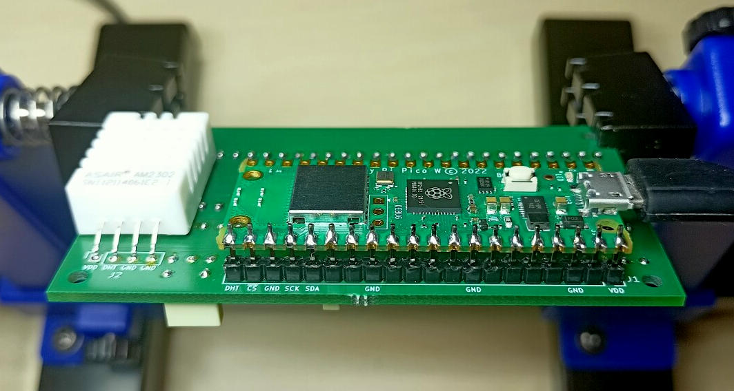
WiFi-clock: NTP client and SNMP agent
Happy Daylight Saving Time!
As a practical joke on inhabitants of the Nordic capital, Summer Time arrived with a mighty snowstorm that brought icy wind and heaps of fresh snow for yet another week. The other remarkable fact about this year’s better-sided transition is that I now have not one, but two different self-made clocks, both having demonstrated their ability to auto-adjust. After the DCF77 radio-based first clock I made last year, this second one is a little different:
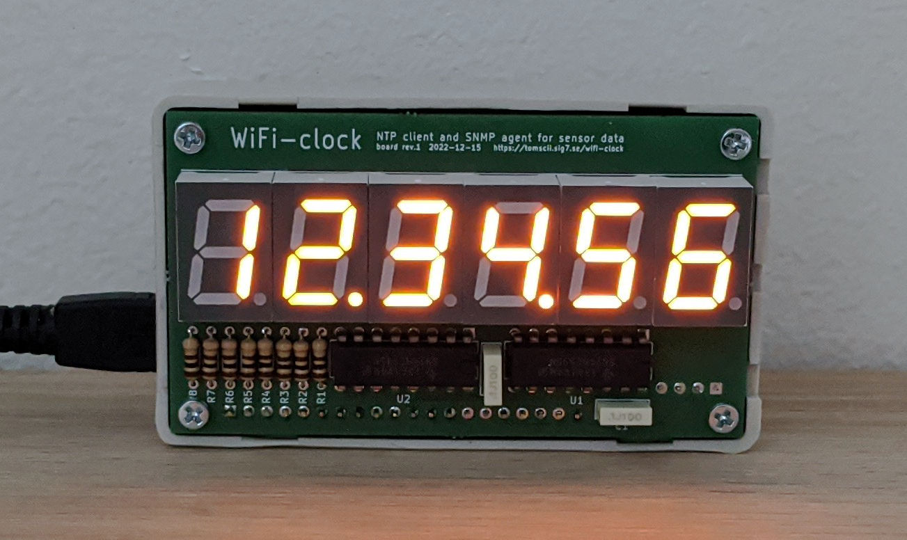
The WiFi-clock caught at the magical 12:34:56 (click to enlarge)
Dubbed the WiFi-clock, this gadget joins my local wireless network (2.4 GHz band of the wireless access point) and obtains the precise time via NTP from a well-known pool of servers. It also measures the temperature and relative humidity with the same type of sensor as its predecessor, but instead of displaying it (which it could well do, I was just lazy) it makes the latest measured values available via SNMP. This, in turn, makes it quite easy to channel that data into μMon, my home-grown monitoring toolkit, yielding graphs of temperature and humidity over time. Here is past week’s indoor weather:
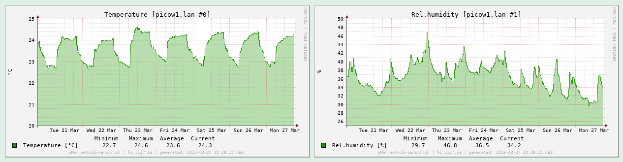
Graph of measurement data in μMon (click to enlarge)
Initial goals and project scope
After some hands-on design and programming experience with Atmel’s 8-bit AVR microcontrollers (as exemplified by the ATmega328P employed in my DCF77 clock), I wanted to move on and learn something different. I chose the Raspberry Pi Pico, a cheap board built around the RP2040 microcontroller. This is a powerful 32-bit dual ARM core with a 133 MHz clock, lots of standard peripherals and GPIO pins. Having written some embedded software for the STM32 many years ago, I now wanted to explore this relatively recent newcomer instead.
I was drawn to the platform due to its high quality documentation (datasheets and specifications as well as implementation guides), lots of code examples and the availability of a software SDK usable in an entirely open source environment with no reliance on some big fat ugly IDE.
The final selling point was the existence of the Pico W, a variant of the Pico board with an Infineon CYW43439 wireless chip providing 802.11n (2.4 GHz) wireless connectivity. Wireless is integrated into the Pico’s C/C++ SDK via the free lightweight TCP/IP stack. It all looked very promising, and at the price point of 95 SEK apiece I could not resist.
After my “rat’s nest experience” with my DCF77 clock, I also decided that I want to avoid a second instance of that at any cost. So I set out to finally level up my game and design a real printed circuit board that can be manufactured for me. That meant learning even more skills, spending even more time – make no mistake, PCB design is a complete art and profession in itself, but as I found out, it is also a lot of fun!
The LED display
Since this is going to be a relatively high-powered circuit anyway (with WiFi and a couple 133 MHz cores), I decided that the low-power aspect was of secondary importance this time. I am going to power the circuit by re-purposing an old 5V phone charger, plugging it into the Pico’s micro-USB port. The Pico will in turn power the rest of the circuit, which is mostly just the LEDs and their drivers.
This generous power design allowed me to use six 7-segment LED digits lined up to form the display. I got CA-type (common anode) ones in a nice orange colour. (A minor annoyance is that there are decimal dots, but no separator colons. I would have used the appropriate LED module if I would have found one, but there was none in stock. This scarcity economy…)
To drive all the LEDs (6 x 8 = 48 in total), I chose the trivial (and usual) time-division multiplexing scheme. Each digit is displayed on its own, one after the other, in a round-robin fashion with a sufficiently high refresh rate that the human eye cannot perceive any flicker. This way, the state of the display fits nicely into 16 bits driven by two 8-bit shift registers: 8 bits for driving the seven segments plus decimal dot, and the rest of the bits to control which of the digits to power with the chosen pattern.
As a natural subdivision, the CA (common anode) pins of the LED displays will get connected to subsequent bits of the upper byte (each to their own), while the lower byte’s bits are distributed to all the LED displays in parallel (one line for each individual segment). So the upper bits will be 1-of-N encoded with active high level, and the lower bits will be set according to the desired digit, encoded active low (since those are the LED cathodes).
That much is trivial, as any first-year student of electrical engineering will surely know. What I did not realise for a while (although started to get enlightened while working on my DCF77 clock) was how simple and easy it was to drive such an arrangement from the MCU side using the SPI peripheral. Sure, I knew about SPI peripherals and how various chips can be hooked up to an MCU with it… but lacking practical design experience, it simply did not occur to me that SPI, at its essence, is nothing but a shift register, so the only thing that is really required to have an “SPI peripheral” is in fact a shift register.
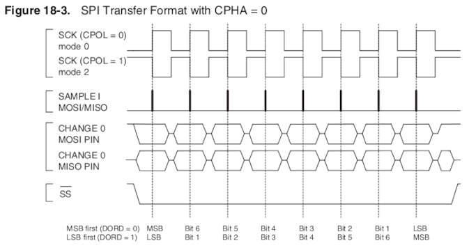
Stolen from the ATmega328P datasheet
The only noteworthy “trick” is controlling the transfer. I realized that the SPI SS (Slave Select) or CS (Chip Select) as they called it on the Pico board, driven low for the duration of the transfer and then released, can be used for latching the shifted-in data onto the output pins. So the output of the shift registers will be stable (holding on to the old values) while the new bits are shifted in, and then at the end of the transfer (rising edge of SS), it gets latched out all at once.
All you have to do to make this happen is tie the SS from the MCU to the register clock input of the 74HC595 and it will just work (with the correct SPI transfer mode settings, etc). After an SPI write on the MCU side, the shift register outputs will change (after a small delay) in parallel. The delay is basically a (very small) constant(ish) time, plus the time it takes to clock out the data with the SPI clock; in my case it’s 16 bits at 16 MHz, so about 1 μs. I could have done the same on the AVR, and I would have spared myself a lot of disassembly reading and instruction cycle counting. Plus, the SPI peripheral runs parallel to the core, leaving the MCU available for other tasks during the transfer.
Oh well, I guess it’s never too late to get better at doing things. So now driving the time-multiplexed LED display, on the software side, boils down to a simple scheduled timer with a fixed period of repetition (let’s say 2 ms), stuffing the next digit (round-robin), appropriately encoded in the above manner, into the SPI. The 2 ms delay means we are operating at an 500 Hz update cycle, but divide that with the number of digits for the full periodicity. I settled on this seemingly high rate for the excellent stability it provides; I don’t want anyone in the room to get headaches from additional flicker.
Breadboard version
As soon as I had my Raspberry Pi Pico SDK and toolchain up and running, I wanted to experiment with an actual circuit while testing various code ideas. A breadboard version was also desired for some fine-tuning (e.g., the size of the current-setting resistors for the LED segments) and validation (is the Pico’s internal pull-up OK with the sensor?), so I built one:
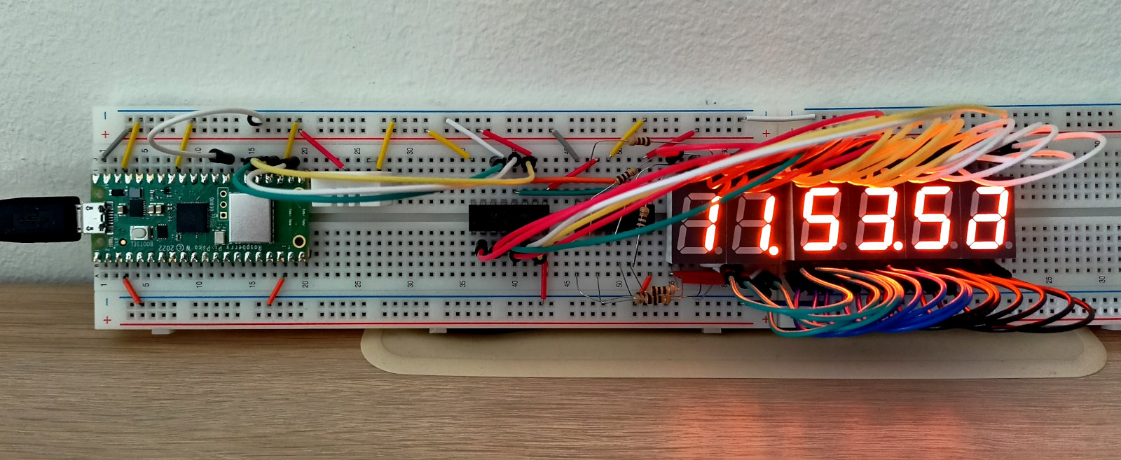
Breadboard version (click to enlarge)
Notice how neat this is (if you discard the lump of wires on the right): there are only three lines (green, white and yellow) connecting the Pico and the ‘595s, visible in the middle left of the image. These three wires constitute the complete display interface between the “compute module” and the “display module”. Yes, that is in fact a one-way SPI connection. No doubt I am re-inventing the wheel, but at least it’s a good wheel!
The complete schematic
Since all the heavy lifting is done by the Pico W, the complete schematic of the rest of the system is actually pretty uninteresting. It is just an implementation of the 16-bit SPI peripheral discussed above for driving the LED digits, plus a connector for the DHT22 temperature and humidity sensor. The most interesting part is shown below; click for the complete sheet or download it in PDF:
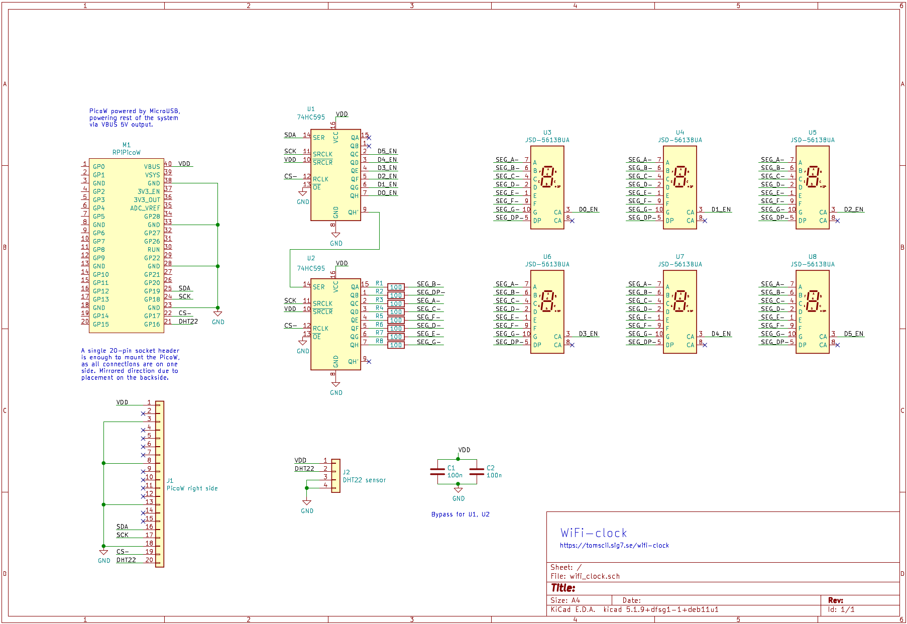
Schematic (click for full sheet), PDF
No surprises there.
Now for the best thing since sliced bread:
A professionally manufactured PCB!
Since I was already well on my way to learning KiCAD while working on my DCF77 project, it was natural that I used it to design the PCB as well, adding pcbnew to my EDA toolbelt. I made the most basic type of board, which is a two-sided board with most of the signals on one side, with power and ground (and any remaining unrouted signals) on the other. Given the relatively low complexity, I managed to route everything with exactly zero vias!
Here is the board layout (edges, silk and technical layers only, plus pads):

PCB layout (click to enlarge)
Two 100 mil pin header connectors, J1 and J2, are placed on the back side of the board and thus mirrored here (with their silk rendered purple instead of cyan). J1, the long one, mounts the Pico W as a daughter board, while J2 is the four-pin layout of the DHT22 sensor.
I slightly violated some courtyard clearances (which the DRC, the Design Rule Checker was eager to point out) in the interest of having the holes aligned on a 100 mil raster, but in practice those components fit perfectly well. I guess I could spend some couple dozen hours tweaking my custom collection of PCB footprints (based on precision measurements of the actual components in my inventory), but I deemed this good enough. Here is how the signal routing (front side copper) turned out:
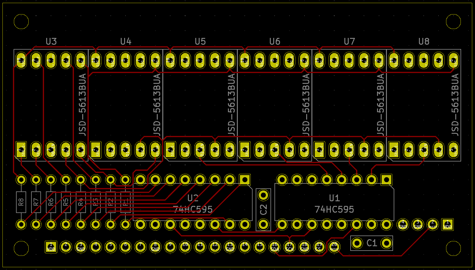
PCB front copper (click to enlarge)
In case you are wondering, the thickness (or rather, thinness) of all signal lines is set to 8 mil (0.2 mm). This is a pretty good starting point; it is sufficiently fine that you will have little trouble wiring up DIP and typical through-hole components (as you can see, I have routed quite a few lines between IC pins). At the same time, it is still safe to manufacture at any standard PCB factory.
Note: If you are designing your own PCB, always check the detailed specifications (usually called Design Rules) for the PCB fabrication process you plan to choose! This applies not only to minimum trace width, but also minimum clearance (necessary gap between separate conductors), clearance from board edge, minimum hole diameter, and typically many more parameters. Time spent studying your PCB factory’s rules and making sure your design fully complies with them is time very well spent!
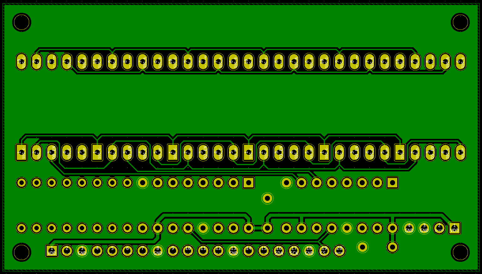
PCB back copper (click to enlarge)
I used the back copper for power distribution and the remaining signals (mostly wiring to connect the segment output to each LED unit in parallel). The rest was filled as a ground plane: even though this is not the type of circuit that would normally justify it, I had to test this feature once I had a grasp on KiCAD’s filled zones. If I would do this again, however, I would certainly do “thermal relief” pad connections instead of the solidly connected pads I did here. Obviously, the ground copper is a very good conductor – of not just electricity but also heat! Hence, soldering to these “solid-grounded” pads becomes a bit challenging.
As a bonus, the KiCAD PCB design tool has an excellent 3D viewer allowing us to inspect our design, even drawing an approximation of some of the components (those that can be matched to its library of 3D models based on their set footprint). Compare this with the topmost image above, and you will see it is pretty good:
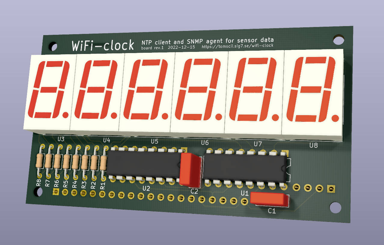
3D viewer with ray tracing (click to enlarge)
I finally ordered manufacturing of the board from Aisler, choosing their lowest tier “Beautiful Boards” service. I went with Aisler after a careful evaluation of several alternatives, due to good feedback on their quality and that they offer manufacturing in prototype quantities within the EU. Here is a link to their PCB Design Rules. Another nice thing about Aisler is that they are capable of taking in your KiCAD PCB project directly, i.e., you don’t have to go through exporting Gerber files, proofing them, and zipping them for upload (as is usual). (N.B.: I am not affiliated with Aisler, but I do believe they deserve your attention if you, like me, want your board manufactured “at home” in Europe instead of China or elsewhere. I also found the price to be very reasonable.)
After the obligatory Long Wait, my boards finally arrived in the post. I was not disappointed – the boards were beautiful indeed! Having uploaded a KiCAD PCB project file a couple weeks ago, there was something magical about seeing it materialized, finally holding a real PCB in my hand. Now, since I had all the parts on the breadboard already, I immediately set out to stuff them into one of the PCBs.
This went like a breeze! All components fit perfectly, and soldering to this board was like a dream. As I quickly found out, a professionally manufactured PCB is the holy grail of non-trivial self-designed circuits. I don’t think I will ever do another circuit without drawing a proper PCB and ordering it – the difference is just enormous and the effort is so worth it!
Oh, and it worked perfectly on the first power-up!
Soldered first board (click to enlarge)
Here you can see the flip side of the first board I made, with the Pico W as daughter board and the sensor on its left. (I later had to re-solder the sensor with longer leads, so I could place it on the outside of the box, after discovering that the measured temperature was consistently higher than expected by 2 to 3 degrees… who would have thought the LEDs would warm up the inside of the box?)
Failings of a software nature
Not everything works as you would expect. Sometimes, I wonder how anything works at all, given the amount of bugs everywhere. The mighty shenanigans frequently boil down to issues on the Dark Side: software. Give up all hope, ye who have put code into production.
WiFi connection (in)stability
The program running on the Pico W developed organically from the NTP example which comes as part of the Pico C/C++ SDK examples collection. This taught me how to program against the lwIP (lightweight IP stack) in a callback-driven style. I did not have any difficulties coding what I wanted; the APIs are quite clear.
One “gotcha” I spent much time on was every now and then, the WiFi connection seemed to break down for no apparent reason. After much poking around, I came up with some code that was able to detect if the wireless connection appeared to go down, and initiate a re-connect. It worked… well, most of the time. The whole thing is a hack that should never be necessary in the first place. Searching for this issue, I found that others had similar troubles as well, and it is usually blamed on the closed source blob that is the wireless chip’s firmware, which is allegedly (and very likely) buggy.
Oh well, I guess that is where the famed openness of the Raspberry Pi Pico platform ends. As I still have not found a perfect cure, I cannot recommend this board (at least the WiFi-part) for anything “serious”.
Later on, I found that if my μMon system keeps polling the device once per minute, that will seriously improve stability. It is as if the network stack in the Pico W would get bored (reach some inactivity timeout) unless there is recurring activity. Alas, comms will still go down sometimes (resulting in a few missed samples every week or so), and while it eventually always “fixes itself”, this is irritating at best and unusable at worst.
I was briefly concerned whether the large ground plane on the base board I designed (which is at most 10 mm from the Pico W daughterboard) could cause any such issues. While I can’t be completely certain, I feel comfortable about it for two reasons: first, the WiFi troubles really look like a software issue. Second, the Pico W antenna is on the outer side (facing “free space” with the enlarged ground plane behind its back), so my feeling is that the antenna should perform at least as well as without the extra ground plane.
Sensor data encoding
I used the same DHT22 temperature and relative humidity sensor as I did in my earlier project, to the point that the manufacturer’s markings on the white package are identical (except the date). In addition, I have tested the sensor below freezing temperatures and had no trouble reading out sensible values (according to the instructions on the Chinese “datasheet”). So I was a bit surprised when, having coded to the same spec with confidence, I got some temperature values on my first freezer test (see below) that looked like completely nonsensical garbage at first: -3276.6 °C (that should have been -0.1 °C, having just crossed below 0). It did not take much staring at that value before I had my suspicions…
Sure enough, the new sensor encodes negative temperatures differently than the (seemingly identical) old one. The old one used the (documented) “sign bit, then absolute value” encoding, while the new sensor is simply outputting a signed integer in two’s complement encoding. While I actually prefer this second encoding, this does not seem documented at all.
The scary bit is that for positive temperatures, there is no difference – both sensors will return similar values. But for a sub-zero temperature such as -7.2 °C, there will be two versions:
| Temperature | Sensor data | Note |
|---|---|---|
| -7.2 °C | 0x8048 |
Sign bit, then absolute value |
| -7.2 °C | 0xffb8 |
Two’s complement |
If you do not actually test your device below zero degrees, you might have an Easter Egg (potentially “exploding” values from the sensor) in your system. And the “datasheet” (if that word can be used here) is apparently worthless.
Software highlights
I wanted to highlight some more interesting parts of the software I wrote for the Pico W.
Daylight Saving Time implementation
Compared to my DCF77 clock on the much more primitive AVR platform, time-keeping is much simplified on the Pico due to the presence of its RTC (Real-Time Clock) module. Upon reception of the current time via NTP, we just set the local RTC to that time, and it will keep ticking. This way, driving the display (showing hours, minutes and seconds) becomes a trivial exercise of reading the RTC for the current values. No actual time-keeping code is needed.
However, NTP does not include timezone information; it only gives us a precise timestamp in UTC. And of course, we want the clock to display our local time. How do we take the (seasonally changing) timezone information into account?
The solution on most computing platforms is something called tzdata
– a timezone database that contains detailed rules for all the
world’s timezones, and is typically updated muliple times per year to
keep it in sync with reality.
That is decidedly not something I wanted to use in this project, so I thought about the easiest way I could solve this myself. The timezone is fixed: Central European Time with or without DST, i.e., CET (UTC+1) or CEST (UTC+2). So we only need a lookup table that will, for any given year, tell us the timestamps (in UTC) of the start and end of DST.
The rules for DST transition dates are pretty simple: transitions happen on the last Sunday of March and last Sunday of October. So the lookup table is just a linear array of timestamps, indexed by the year: for the i-th year stored in the table, the timestamps at array offsets 2i and 2i + 1 will contain the start and end of DST.
Once we have such a table, it is most natural to use it on reception of the NTP data: we know the year from the response, and based on that, it is trivial and computationally cheap to look up whether the current UTC timestamp is within the given range for DST. If it is, apply another hour of offset on top of the fixed hour. Use the result (now in local time) to set the RTC.
Having designed this simple scheme, I considered generating the lookup table on demand at first use, or once on power-up. In the end, I settled for an even easier way: just pre-generate the table and compile it in. This way, the calendrical calculations (which day is the last Sunday of March in a given year?) can be performed by host software that can be much more powerful, can be written in whatever language, or can use whatever library that conveniently solves the task.
To demonstrate this idea, I wrote the DST table
generator
in Common Lisp. The program, when run, produces the header file
dst_table.h that becomes part of the sources to be compiled for the
Pico W. This is how the generated include file looks:
/* generated by dst_table.lisp */

static int dst_table_start = 2020;
static int dst_table_years = 80;
static time_t dst_table [] =
{
   1585443600, 1603587600,  // 2020-03-29 -- 2020-10-25
   1616893200, 1635642000,  // 2021-03-28 -- 2021-10-31
   1648342800, 1667091600,  // 2022-03-27 -- 2022-10-30
   1679792400, 1698541200,  // 2023-03-26 -- 2023-10-29

   ...

   4046979600, 4065123600,  // 2098-03-30 -- 2098-10-26
   4078429200, 4096573200,  // 2099-03-29 -- 2099-10-25
};
The Common Lisp program generating this is less than 60 lines of the most trivial kind of Lisp. I am convinced this is a good division of labour. Generating code is a technique I like to use, and Common Lisp is probably the best language to use for that purpose.
I am also highly confident that 80 years of coverage will be more than enough for this project, but there is nothing magical about that – all time handling is 64-bit already.
An SNMP agent
Given that the device is already “online” for the purpose of obtaining a precise timestamp via NTP, it was only natural to equip the software with support for serving sensor data over the network as well.
But in what format? I briefly considered a few options. First, some bespoke (custom and simple) request and response protocol over TCP, perhaps binary or maybe textual… Programming this would not have posed any challenge or excitement. Of course, I would have had to do the host counterpart (the “client” program that queries the device) as well. Ultimately, I found this idea too boring.
Second, I thought maybe I would run a webserver on the Pico, so a
standard HTTP query could be used to request and then receive the
data. This looked a bit more interesting; at least, one could use
curl instead of a bespoke client. On the downside, even with a
minimal set of HTTP headers, the overhead looked unnecessarily large.
Then it occurred to me that there is already a very capable, efficient, flexible and well documented protocol to do what I want. Yes, it’s called SNMP, which has gotten associated with a rather steep curve of complexity (despite Simple in its name). Even though it did not look very appealing at first, the more I thought about it, the clearer it became that if I wanted my device to be interoperable with clients I did not write, SNMP was actually the best option.
I guess part of the reason for today’s aversion to SNMP is that it is one of those old telco-era designs with standards documents in the thousands of pages, mandating a mountain of (perceived) complexity. On the flip side, actual problems were solved by the people coming up with it, and solved in a close to optimal way. In those days software system design was a Serious Activity not to be rushed but carefully documented, and being (or looking) Agile was not a priority. While the lacking appeal of SNMP to today’s hipster programmers can be well understood, I believe it is more about fashion and “culture” than anything else. Parts of SNMP are complex, because it aims to be flexible: the ASN.1 data definition language and the MIB (managed information base) both make it adaptable to basically anything. SNMP was mostly designed in an era of scarce computer resources: CPU cycles, bytes held in memory or sent over the network were all at a premium. Something like JSON would have looked ridiculous at the time.
I find it a rather interesting techno-historical artifact how we keep reinventing simpler subsets and alternatives of e.g., ASN.1 instead of embracing it, when in fact ASN.1 has most of the features (and more) of several more modern IDLs such as Avro, Thrift, Protobufs, flatbuffers and many similar projects, all in one unified framework. The different encodings such as BER, DER (plus XML, etc.) were also invented for (at the time) good reasons, and their designs were sound within their scopes and boundaries. Of course, it is an enormous pile of complexity if one aims to implement everything, but that is almost never necessary. For example, SNMP only uses a small subset of ASN.1 for defining its MIB, and its on-the-wire PDU format is restricted to one possible encoding.
So how hard would it be to make my gadget respond to an SNMP query? Spoiler alert: I managed to write a simple but highly useful read-only SNMPv2c agent in two very relaxed afternoons, in the end taking up about 300 lines of C code. I was pleasantly surprised by this result, as I did not think I would make it under a thousand (and such estimates are usually off in the other direction). It also went way easier than I thought it would to make it work. So I reflected a little more on this… and at the risk of upsetting some (insecure) people, I will say that processing SNMP is basically just consuming and producing small UDP packets; any competent C programmer should be able to figure it out. It feels scary, but it’s not that hard. (Let’s just ignore SNMPv3 and hope that you never have to deal with that.) While we are getting surrounded by a world of auto-scaling Kubernetes clusters and “our cloud migration strategy” is a regular item on the agenda of many CTOs, here’s a little secret: SNMP(v2c) is not hard at all. It’s a (relatively) simple, standard, old protocol you (yes, you) could use for a lot of things. You can depend on it, because it won’t go away. Once you integrate with it, it will serve you with no surprises and no churn down the road, because it is done.
So as I said, about 300 lines of reasonably readable C code, which is
next to nothing! At the same time, the agent correctly authenticates
and responds to queries (both simple Get and GetNext, i.e., snmp
walk, queries are supported) and understands the object hierarcy
under the “Entity Sensor MIB”. I can “walk the whole MIB” from any
standard SNMP client, e.g., Net-SNMP on Linux:
$ snmpwalk -v2c -cpublic picow1.lan .1.3.6.1
iso.3.6.1.2.1.99.1.1.1.1.1 = INTEGER: 8
iso.3.6.1.2.1.99.1.1.1.1.2 = INTEGER: 9
iso.3.6.1.2.1.99.1.1.1.2.1 = INTEGER: 9
iso.3.6.1.2.1.99.1.1.1.2.2 = INTEGER: 9
iso.3.6.1.2.1.99.1.1.1.3.1 = INTEGER: 1
iso.3.6.1.2.1.99.1.1.1.3.2 = INTEGER: 1
iso.3.6.1.2.1.99.1.1.1.4.1 = INTEGER: 240
iso.3.6.1.2.1.99.1.1.1.4.2 = INTEGER: 372
iso.3.6.1.2.1.99.1.1.1.5.1 = INTEGER: 1
iso.3.6.1.2.1.99.1.1.1.5.2 = INTEGER: 1
iso.3.6.1.2.1.99.1.1.1.6.1 = STRING: "x0.1 *C"
iso.3.6.1.2.1.99.1.1.1.6.2 = STRING: "x0.1 %RH"
iso.3.6.1.2.1.99.1.1.1.6.2 = No Such Object available on this agent at this OID
I have also tested the code with OpenBSD’s SNMP client, which is slightly less forgiving about the minimum-length rule of encoding integers. To only get the non-static part of the MIB (i.e., the measurement values) in a single query-response:
$ snmpwalk -v2c -cpublic picow1.lan .1.3.6.1.2.1.99.1.1.1.4
iso.3.6.1.2.1.99.1.1.1.4.1 = INTEGER: 240
iso.3.6.1.2.1.99.1.1.1.4.2 = INTEGER: 371
Interpretation of the values is trivial: temperature is
24.0 °C and relative humidity is 37.1%. It also helps that
the Entity Sensor MIB is something I did not come up with – yes,
it is an existing standard MIB. Plus, the strings given as the Display
Units of these variables have the clues x0.1 *C (tenth of °C)
and x0.1 %RH (tenth of a percent of relative humidity). Having these
features clearly shows that SNMP was designed to facilitate data
interchange in an open (inter-vendor) environment.
SNMP is definitely not without its shortcomings, and there are of course lessons to be learned (both good and bad) from the solutions that succeeded it. What I’m saying is two things. First, don’t be afraid to use SNMP. Second: SNMP can be implemented in a much smaller footprint than you might be led to believe.
LED brightness control
Having had the WiFi-clock in the living room for a couple months, I had an extra idea for improving the device: could I make the brightness of the LED display controllable? Ideally, by supplying a brightness percentage between 0 and 100. With that feature, I could program the clock to dim the brightness at a certain hour in the evening.
As I had not made any provisions for this when designing the electronics, it had to be implemented purely in software. It naturally occurred to me that modifying the scheduled timer driving the display (the one which puts up the next digit via SPI every 2 ms) was the way to go. First, I thought I would inject “black” frames, i.e., every N timer period would include one (or several) where all the segments of the display would be off. However, the brightness will only match expectations in average over a longer period: if there is one “black frame” in a hundred, that means 99 frames, or a consecutive 198 ms, will be on full brightness. That won’t work.
A better way, providing superior granularity, is to simply introduce a frame-end blanking timer. This is set to a time proportional to the desired brightness. For example, if we aim for a brightness of 10%, we want the display to be on for the first tenth of the 2 ms frame, or 200 μs. If we want a brightness of 90% instead, we set the timer length to 1.8 ms. On each display update, we start the frame timer and when it fires, we output the “black” frame which will turn off all LEDs until the next display update. We have the luxury of doing this as even with the seemingly high refresh rate of every 2 ms, we still have a lot of processor cycles to use. Scheduling another timer is virtually no cost on this hardware.
One obvious corner case is maximum brightness (which is most of the time during the day, i.e., when we are actually going to look at the clock, so it is kind of important). But correct handling of this is trivial: if the desired brightness equals the maximum value of 100, we simply do not start the frame-end timer at all.
With this addition, the WiFi-clock goes from full brightness to a discreet orange glow in the evening, so people glancing at it in the darkness of the night won’t be woken up even more than they already are. At seven in the morning, full brightness strikes again as the day starts. To me, this is part of the reason to own the gadgets surrounding me: I can make them behave precisely how I want them to. No commercial off-the-self device would give me such power over its workings!
Test drive: Measuring the freezer
Have you ever measured how cold your freezer is… via SNMP over WiFi? Seemed like a cool idea to me… So I hooked up the device to a USB power bank and wrapped the whole bunch in a resealable plastic bag with as little air trapped as possible, then placed the bag in the freezer. Then it was only a matter of watching μMon and waiting:
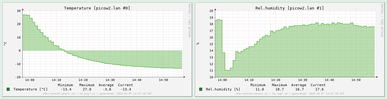
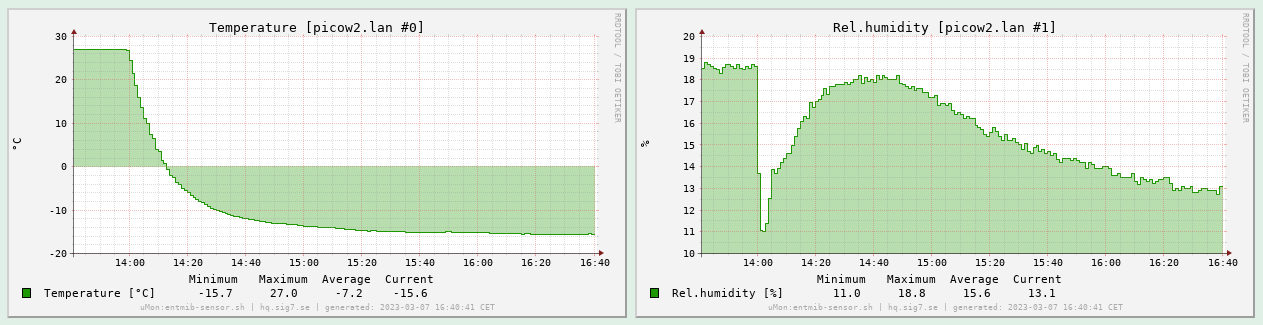
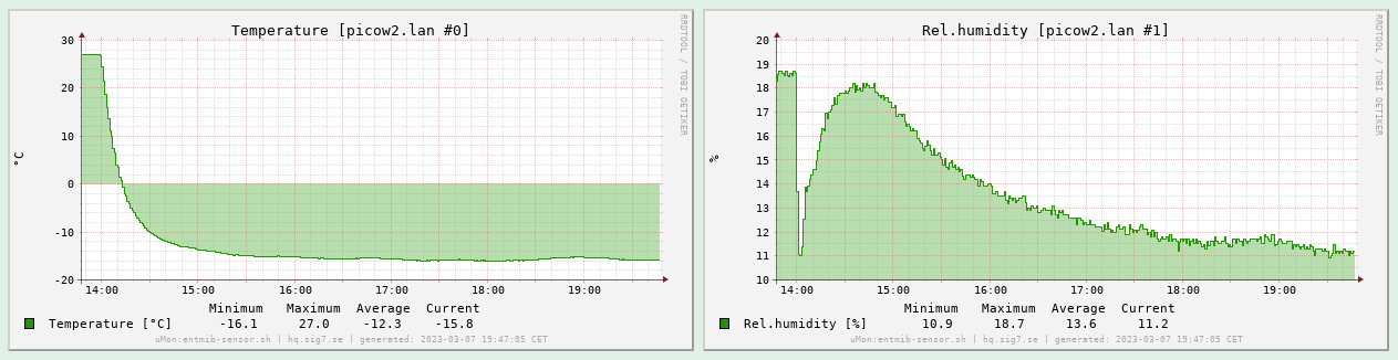
Cooling down… (click to enlarge)
Considering the small size of the gadget, it actually surprised me how long it took to reach full thermal equilibrium: almost two hours!
I reckon the measured temperature in these graphs is ~2 degrees above reality (see above note on the warming effect of the LEDs), putting the stable temperature inside the freezer squarely at its nominal -18 °C.
Conclusion
The WiFi-clock has been in non-stop operation in my living room with its sensor data fed into μMon since mid-November 2022. Apart from the very annoying (but ultimately rare) disturbance to its wireless connection (discussed above), the device has been operating flawlessly. In particular, time is displayed with perfect accuracy at all times and the DST auto-switchover is now proven to work as well.
Hardware cost and bill of materials
Just as with my previous hardware project, I am sharing with you a listing of components and other costs associated with this build. Here again, please keep in mind that the cost of components heavily depends on the quantity, and I am buying everything in the smallest possible quantities: single pieces or a few at most. If this was produced by some electronics factory, the per-unit cost would be a small fraction of the total amount below. Keep that in mind when you are looking at fancy overpriced electronics to buy: this is fundamentally cheap technology! Yes, that applies even to the PCB: just look how little it cost to have three(!) identical custom boards manufactured. (Three, because that is the minimum order quantity. I’m still amazed that there are manufacturers who put up with orders of three boards!) If I would have wanted three thousand, it would have cost much less still.
| Component | Unit price (SEK) | Quantity | Subtotal (SEK) |
|---|---|---|---|
| USB power (old phone charger) | free (YMMV) | 1 | - |
| Raspberry Pi Pico W | 95.00 | 1 | 95.00 |
| DHT22 sensor | 99.00 | 1 | 99.00 |
| 7-segment LED-display 14mm orange CA | 10.00 | 6 | 60.00 |
| 74HC595 | 5.90 | 2 | 11.80 |
| Polyester cap R82 100nF 100V | 3.00 | 2 | 6.00 |
| Resistor 100Ω 0.25W 5% | 1.00 | 8 | 8.00 |
| 100 mil pin header, breakable, 40 pins | 9.00 | 1 | 9.00 |
| Plastic instrument box 50x84x20mm | 39.00 | 1 | 39.00 |
| Metal distancer screw M2.5 11mm | 7.50 | 4 | 30.00 |
| Screw M2.5 x 6 mm | 2.85 | 4 | 11.40 |
| PCB manufacturing order | EUR 13.18 | 1 | ~150.00 |
| Total: ~520.00 |
Since the price of PCB manufacturing was quoted (and paid) in Euros, the conversion to SEK is an approximation as it depends on the ever-fluctuating exchange price. Again, please note that for the given cost I received three boards to my door – if I amortize that cost to three devices, that is about 50 SEK per gadget for a professional PCB, carrying components worth another 370 SEK. Or to put it another way, the PCB (amortized) is about 12% of the unit cost. I find that price well worth paying to put my design in a much more professional form.
Source code repo
You are welcome to check out the repository containing all the source code, KiCAD hardware design and miscellaneous notes and documents I collected while working on this project. It is now published online with all source code licensed under the terms of the very permissive BSD license.