DiGenO is a Distributed Genetic Optimizer framework in Erlang. It implements a steady state evolutionary algorithm, parallelized over an arbitrary number of loosely coupled computational nodes (Erlang cluster).

The goal of DiGenO is to make it easy for you to formulate your genetic optimization problem, and then do everything else so you don’t have to. There are three example problems formulated as DiGenO callback modules ready for you to try right away. We will introduce DiGenO by taking a look at these problems and their example solutions. Get the source if you want to follow along.

Anatomy of a DiGenO optimization problem

To optimize with DiGenO, the problem must be embodied by a callback module implementing a certain interface. The functions of this interface are called by the DiGenO framework throughout the optimization process.

The most important functions are the following. You should consult src/digeno_callback.erl for the full specification.

%% Generate a new instance
-callback generate() ->
          Instance :: term().

%% Evaluate the fitness of an instance. Result must be a term
%% interpreted by callbacks `fitness' and `dead_on_arrival'.
-callback evaluate(Instance :: term()) ->
          EvalResult :: term().

%% Compute the fitness of a given instance based on its evaluation
%% result. This must return a floating point number that is greater
%% (more positive) for better instances.
-callback fitness(Instance :: term(), EvalResult :: term()) ->
          Fitness :: float().

%% Mutate an instance.
-callback mutate(Instance :: term()) ->
          MutatedInstance :: term().

%% Combine two instances into a new one. Also called crossover in GA terms.
-callback combine(Instance1 :: term(), Instance2 :: term()) ->
          Instance :: term().

Since we use the dynamically typed Erlang language, a word about data types is in order. An instance can be any data structure; the same is true for the evaluation result of an instance. You can choose any meaningful representation that suits your problem.

However, there must be a mapping from the evaluation result to a floating point fitness number that is greater for better instances: those with more desirable properties or representing a more fitting solution to the problem. DiGenO does not care what the instances and the results of evaluation are, but it ranks instances by fitness.

Problem 1: String evolution

This is the first and most trivial example, in fact the proverbial “Hello World!” of genetic optimization problems. The goal is to evolve randomly generated garbage into a predefined string. This problem is of no use outside the scope of testing the solver itself.

Here follows the bulk of the callback module defining this problem. The less interesting parts are omitted; please check src/example_string.erl. It should also be noted that the DiGenO utility module utils contains several useful facilities for writing functions that operate in a probabilistic manner (e.g. use random selection).

-define(TARGET, "Now is the time for all good men "
                "to come to the aid of their party!").

generate() -> gen_random_string([], length(?TARGET)).

mutate(Instance) ->
    Pos = random:uniform(length(Instance)),
    utils:change_item(Pos,
                      lists:nth(Pos, Instance) + utils:crandom([1, -1]),
                      Instance).

combine(I1, I2) ->
    Pos = random:uniform(length(I1)),
    I1a = lists:sublist(I1, Pos),
    I1b = lists:nthtail(Pos, I1),
    I2a = lists:sublist(I2, Pos),
    I2b = lists:nthtail(Pos, I2),
    utils:crandom([I1a ++ I2b, I2a ++ I1b]).

evaluate(Instance) -> distance(Instance, ?TARGET).

fitness(_Instance, 0) -> 2.0;
fitness(_Instance, EvalResult) -> 1.0 / EvalResult.

%% private functions

random_char() -> $  + utils:grandom(95). %% ascii printable

gen_random_string(Str, 0)   -> Str;
gen_random_string(Str, Len) -> gen_random_string([random_char() | Str], Len-1).

dif({A, A}) -> 0;
dif({A, B}) -> (A - B) * (A - B).

distance(S1, S2) -> lists:sum(lists:map(fun dif/1, lists:zip(S1, S2))).

Needless to say: instances in this problem are strings. Generating a new instance is thus equal to generating a random string with the given length (the length of the target). We could play with allowing varying string lengths here; this would complicate our evaluation function but would not change the fundamentals of the problem. This is intended to be the simplest possible example, so all instances are of a fixed length that matches the length of the desired target.

Mutating an instance is done by choosing a position in the string and altering the character at that position to either the previous or the next character (ASCII code-wise). So mutations are pretty gradual.

Combining two instances (frequently called crossover in the literature) is done by choosing a random position at which both strings are cut. The combined instance is then either the first part of the first string followed by the second part of the second string, or the first part of the second string followed by the second part of the first string. The choice is random.

Evaluation of an instance is done by summing the squared differences in character values between the instance and the target string. This integer number is the evaluation result itself; it is converted to fitness via taking its reciprocal. This will make instances with less distance from the target more desirable (greater fitness), which is exactly what we want. In case there is no difference, the fitness is defined to be 2.0, which is greater than the greatest fitness for any nonzero evaluation result (1.0).

Evolution

This problem has a clear goal and it is trivial to decide when it is reached. For this reason the callback module can configure DiGenO to use a fitness threshold to terminate the process. This is accomplished by the fitness_target in the configuration returned by the get_config() callback function.

get_config() -> [{population_size, 100},
                 {fitness_target, 2.0},
                 {display_decimator, 100}].

The evolution process looks like this:

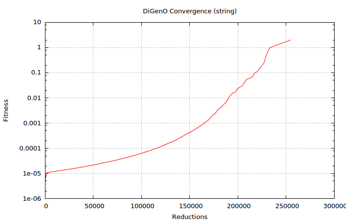
It is interesting to see how the process speeds up (even on a logarithmic scale) as instances closer and closer to the target are evolved from the initially generated “random noise”.

Problem 2: Curve fitting

A similar problem, but actually useful to solve, is evolving coefficients of a polynomial with the goal of fitting the polynomial to some predetermined data. This data is either given by an analytical function or a set of “measurement” points. We choose to use data points, and formulate the problem as follows:

Given an integer N and a set of data points [{X, Y}], determine the coefficients of a univariate polynomial function of degree N that best fits the set of data. Let the minimized error metric be the sum of squared differences.

This example evolves a polynomial of degree N=7, to approximate the function sin(x) over the range [-π, π], represented by precomputed data points in that range.

Instances are polynomial functions of the form:

They are represented by a list of their coefficients:

[a0, a1, a2, ... a7]

We expect the solution to this problem will converge towards

[0, 1, 0, -0.166666, 0, 0.008333, 0, -0.000198]

which contains the polynomial coefficients corresponding to the Taylor expansion of sin(x):

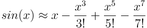
This is our best idea of what we should get out of DiGenO. We’ll return to the accuracy of this approximation a bit later.

Here’s the meat of our problem callback (find the whole source in src/example_curve.erl):

generate() -> random_poly(?DEGREE).

mutate(Fn) -> mutate(Fn, utils:grandom(?DEGREE)).

combine(Fn1, Fn2) ->
    [utils:crandom([Ai, Bi]) || {Ai, Bi} <- lists:zip(Fn1, Fn2)].

evaluate(Fn) -> eval_error(Fn, data()).

fitness(_Fn, 0) -> 2.0;
fitness(_Fn, Result) -> 1.0 / Result.

To make this work, we need a few helper functions. First, let’s look into how instances are generated and mutated.

random_poly(N) -> [random_coeff() || _P <- lists:seq(0, N)].

random_coeff() -> utils:crandom([-1, 1]) * random:uniform().

%% mutate N times in a row to allow changing different coefficients at once
mutate(Fn, 0) -> Fn;
mutate(Fn, N) ->
    I = random:uniform(length(Fn)),
    Ai = lists:nth(I, Fn),
    NewAi = adjust_coeff(Ai),
    mutate(utils:change_item(I, NewAi, Fn), N-1).

adjust_coeff(A) ->
    case utils:crandom([nudge1, nudge2, mag, inv, sign, set0, set1, rand]) of
        nudge1 -> A * utils:crandom([0.2, 0.3, 0.5, 0.7, 1.4, 2.0, 3.0, 5.0]);
        nudge2 -> A * utils:crandom([0.9, 0.99, 0.999, 0.9999, 1.1, 1.01, 1.001, 1.0001]);
        mag    -> A * utils:crandom([0.0001, 0.001, 0.01, 0.1, 10, 100, 1000, 10000]);
        inv when A /= 0.0 -> 1.0 / A;
        inv    -> 0.0;
        sign   -> -A;
        set0   -> 0.0;
        set1   -> 1.0;
        rand   -> random_coeff()
    end.

When mutating, we define a few different ways of changing a coefficient. We do this so different interesting adjustments can take effect. We also do this a random number of times, so more than one coefficient may get adjusted in one mutation. This is so that the optimization does not get stuck in local minima. However, the number of mutations done is generated via utils:grandom/1, which will generate a number with a power law decaying probability function, so 1 is much more probable than 2, which is more probable than 3, and so on. Thus most mutations will in fact consist of one or at most a few adjustments.

Finally, let’s look at how we evaluate an instance. Remember, an instance is just a list containing the coefficients of the polynomial.

eval_error(Fn, Data) ->
    Errors = [eval_fn(Fn, X) - Y || {X, Y} <- Data],
    lists:sum([E*E || E <- Errors]).

eval_fn(Fn, X) ->
    {Y, _} = lists:foldl(fun(Ai, {Acc, Xi}) ->
                                 {Acc + Ai * Xi, X * Xi}
                         end, {0.0, 1.0}, Fn),
    Y.

And where does Data passed into the call to eval_error/2 come from? That is the reference data we are fitting, and is generated by the function data/0. It could be your latest measurement, but for the sake of simplicity (and reproducibility) we generate it like this:

data() ->
    mk_data(fun(X) -> math:sin(X) end,
            {-math:pi(), math:pi()},
            100).

mk_data(Fun, {StartX, EndX}, NumPoints) ->
    Delta = (EndX - StartX) / (NumPoints - 1.0),
    mk_data(Fun, StartX, Delta, NumPoints-1, []).

mk_data(Fun, StartX, _Delta, 0, Acc) ->
    X = StartX,
    [{X, Fun(X)} | Acc];
mk_data(Fun, StartX, Delta, NumPoints, Acc) ->
    X = StartX + NumPoints * Delta,
    mk_data(Fun, StartX, Delta, NumPoints-1, [{X, Fun(X)} | Acc]).

Well, that was not that much code. It is also fairly elegant. But that’s all that is needed to do some curve fitting with DiGenO. It would also be fairly trivial to expand our universe of approximators to include a rich assortment of (recursively defined, thus open-ended) possible functions, as opposed to only polynomials of a fixed degree. But let’s leave that as an exercise to the aspiring user…

Evolution

This is an open-ended problem, since there is no obvious metric of when the evolved instance is “ready” or “good enough”. (In case this was a real problem, though, a sensible error threshold could be derived from the real world constraints that apply.) In any case, the solution may asymptotically converge towards an optimum through a very, very long stretch of continuous improvements.

After 985367000 (almost 10⁹) reductions, the evolution seems fairly converged judging from the very slow rate it is still progressing. It seems fair to terminate the process at this point. This is how best fitness changed over reductions:

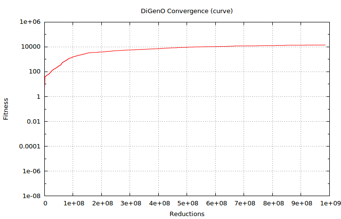
After ~10⁹ reductions, our best instance is:

Candidate = [0, 0.996808, 0, -0.163692, 0, 0.007556, 0, -0.000122].

Compare that with our a priori postulated best instance:

Postulate = [0, 1, 0, -0.166666, 0, 0.008333, 0, -0.000198].

The numbers are pretty close, but not too close. One would expect them to be even closer; it feels suspicious why they aren’t. How does the error metric look like? Let’s evaluate these instances manually to see their sum squared errors compared to sin(x) at a hundred values of x:

> example_curve:evaluate(Candidate).
8.513210195863747e-5

> example_curve:evaluate(Postulate).
0.034772015847635604

Wait, is our evolved instance actually better than the postulated best possible instance? Better by no less than three orders of magnitude lower sum squared error?

The answer is a resounding yes. Reason: we only took a finite number of terms from the Taylor series of sin(x). And as you well know, a Taylor series only represents the function’s value in case the whole (infinite) series is taken into account. By truncating the series at a mere seven degrees, we leave a lot of error in the approximation. And as it turns out, once we stick to approximating with exactly seven degrees, there are better solutions.

Moral of the story: be careful what you optimize for, because you might just get it.

Problem 3: Travelling Salesman Problem

The third and last example problem that ships with DiGenO is the classic Travelling Salesman Problem (hereinafter called TSP). This is a combinatorial optimization problem that is in fact very solvable via a genetic optimization approach.

We are interested in the minimal distance route between 21 Swedish cities: Falun, Gävle, Göteborg, Halmstad, Härnösand, Jönköping, Kalmar, Karlskrona, Karlstad, Linköping, Luleå, Malmö, Nyköping, Stockholm, Umeå, Uppsala, Visby, Västerås, Växjö, Örebro and Östersund. The cities are represented with integers starting with 1, assigned to the cities in the above order.

The input to TSP is a distance (cost) matrix between a number of cities (edges). The goal is to find a cycle in the graph that yields minimal distance (cost) when used to traverse each city exactly once.

To make the problem more realistic, we store the complete distance matrix (in kilometers) for the actual driving distance between any two city, taking into account the existing public road network in Sweden. This matrix of distances is trivially given by city_dist/2 (see src/example_tsp.erl), which looks like this:

city_dist(1, 2) ->  91;
city_dist(1, 3) -> 461;
city_dist(1, 4) -> 572;
...
city_dist(2, 3) -> 518;
city_dist(2, 4) -> 673;
...
city_dist(20, 21) -> 546;

city_dist(A, B) when A > B -> city_dist(B, A).

Instances of our genetically optimized solution are permutations of the order of cities, represented as lists of integers. Permutations define a cycle, meaning that in addition to the route between cities adjacent in a list, the first and last city in the list are also connected. For this reason, the cycle can start anywhere (the problem is invariant to rotation). We will print our permutations always rotated to begin with Stockholm (number 14).

So let’s take a look at the callbacks defining TSP (see src/example_tsp.erl):

-define(NUM_CITIES, 21).

generate() -> utils:permutation(lists:seq(1, ?NUM_CITIES)).

Well, we delegated the task to a function in DiGenO’s utils that takes a list of items and returns those items in randomized order, creating a random permutation of the original list.

Let’s look at mutation and combination:

mutate(P) ->
    %% Swap two randomly chosen cities
    I1 = random:uniform(?NUM_CITIES),
    I2 = random:uniform(?NUM_CITIES),
    if I1 =:= I2 -> mutate(P);
       true ->
            City1 = lists:nth(I1, P),
            City2 = lists:nth(I2, P),
            P0 = utils:change_item(I1, City2, P),
            utils:change_item(I2, City1, P0)
    end.

combine(P1, P2) ->
    %% Choose a random point to cut P1.
    %% Take the items before the cut as they are;
    %% take the rest of the items but in the order they appear in P2.
    Idx = 1 + random:uniform(?NUM_CITIES-2),
    P1Rest = lists:nthtail(Idx, P1),
    lists:sublist(P1, Idx) ++ [I || I <- P2, lists:member(I, P1Rest)].

The combine operation must return a valid permutation, so the usual “naive” crossover method of splicing both instances and gluing them together in a different order won’t work. The resulting list won’t correspond to a valid permutation; some cities will be visited twice, others not at all. So a slightly more clever scheme is needed to arrive at a valid result that still carries information from both “parents”.

I find it remarkable that the combine operation takes three lines to describe in English and three lines in Erlang. The lines of English are in fact longer, if only marginally so. There is no “magic” subroutine called here, so the expressive power of Erlang seems to match that of English in this problem domain.

Lastly, we need to be able to evaluate any permutation. This is trivial: we just sum the distances between adjacent cities in the list, and add to that the distance between the first and last city, which closes the cycle.

evaluate([FirstCity|_] = P) ->
    F = fun(City, {undefined, AccDist}) ->
               {City, AccDist};
           (City, {PrevCity, AccDist})  ->
               {City, city_dist(City, PrevCity) + AccDist}
        end,
    {LastCity, PathDistance} = lists:foldl(F, {undefined, 0}, P),
    PathDistance + city_dist(FirstCity, LastCity).

Again, shorter paths are better, so we create a fitness function based on the reciprocal.

fitness(_P, 0) -> infinity;
fitness(_P, Result) -> 1.0 / Result.

As already mentioned, we print permutations rotated so it always begins with Stockholm (city number 14). This is accomplished via the following code:

format(P) ->
    string:join([integer_to_list(Pi) || Pi <- rotate(P)], " ").

format_result(Result) -> io_lib:format("~B", [Result]).

rotate(P) ->
    %% Rotate cycle to start with Stockholm
    Idx = length(lists:takewhile(fun(E) -> E /= 14 end, P)),
    rotate(P, Idx).

rotate(P, Idx) ->
    lists:nthtail(Idx, P) ++ lists:sublist(P, Idx).

And that’s all we need! Finding the solution is only a matter of seconds running DiGenO.

As it turns out, the optimum path is 3886 km long and is described by the permutation:

14 16 2 5 15 11 21 1 9 20 18 13 10 6 3 4 12 19 8 7 17

This encodes a cycle through the cities in the following order: Stockholm – Uppsala – Gävle – Härnösand – Umeå – Luleå – Östersund – Falun – Karlstad – Örebro – Västerås – Nyköping – Linköping – Jönköping – Göteborg – Halmstad – Malmö – Växjö – Karlskrona – Kalmar – Visby – Stockholm. Nice trip!

Evolution

Look at that convergence:

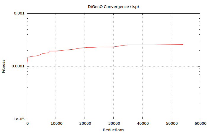
Already after ~35k reductions, DiGenO has a solution so close to the optimum that it is practically the same. Definitely “good enough” if hitting the mathematically exact optimum is not required. Fortunately, real world problems tend to have this property of “good enough is good enough”.

The solution is fully converged after ~55k reductions. Although the exact numbers will vary from run to run, this is clearly the kind of problem that makes genetic algorithms shine.

Interface illustration

This is a screenshot of DiGenO running with the display_vt100 display callback after solving the above TSP example. The convergence listing corresponds to the above graph.

DiGenO running with callback module: example_tsp


Reductions: 108160
Population: 1000

           Fitness      Result   Instance
Worst:     0.00020        4977   14 17 7 8 12 4 3 19 10 13 20 16 9 18 1 21 11 15 5 2 6
 Best:     0.00026        3886   14 17 7 8 19 12 4 3 6 10 13 18 20 9 1 21 11 15 5 2 16


Convergence
         0  9.8000784e-5      4294  1.6321201e-4      22997  2.2779043e-4
         2  1.0643960e-4      5283  1.7328019e-4      25134  2.3068051e-4
        11  1.0956503e-4      7373  1.8024513e-4      29612  2.3174971e-4
        30  1.2043840e-4      7596  1.8092998e-4      31726  2.3929170e-4
        92  1.2537613e-4      7670  1.9387359e-4      31815  2.4137099e-4
       221  1.4259233e-4     10340  1.9474197e-4      32961  2.4551927e-4
       229  1.4841199e-4     12938  2.0177563e-4      34967  2.5555840e-4
      2222  1.5540016e-4     15590  2.0785699e-4      43868  2.5562372e-4
      3067  1.5593326e-4     18460  2.2109220e-4      54078  2.5733402e-4
      3379  1.5750512e-4     21002  2.2758307e-4


Worker nodes (4)
digeno_worker@localhost.localdomain (4)

In this case, DiGenO’s automatic convergence detection stopped further GA execution after a sufficiently large number of reductions without advancing the best fitness. This auto-detection is not foolproof, so you might want to keep it turned off most of the time. Consult digeno_callback:get_config/0 for documentation.